> 2021年04月25日信息消化 ### 每天学点机器学习 #### Week3 Logistic Regression ##### Classification and Rresentation 让我们改变Hypothesis方程形式为以满足 $0 \leq h_\theta (x) \leq 1$ > let’s change the form for our hypotheses $h_\theta (x)$ to satisfy $0 \leq h_\theta (x) \leq 1$. This is accomplished by plugging $\theta^Tx$ into the Logistic Function. Sigmoid Function, also called the Logistic Function. $h_\theta(x)=g(\theta^Tx)$ $z=\theta^Tx$ $g(z)=\frac{1}{1+e^{-z}}$ The following image shows us what the **sigmoid function** looks like: 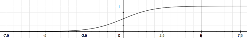 这里显示的函数g(z)将任何实数映射到(0, 1)区间，使得它在将一个任意值的函数转化为更适合分类的函数时非常有用。 > The function g(z), shown here, maps any real number to the (0, 1) interval, making it useful for transforming an arbitrary-valued function into a function better suited for classification. ###### Interpretation of Hypothesis Output $h_\theta(x) = P(y=1|x;\theta)= 1-P(y=0|x;\theta) $ "Probability that y=1, given x, parameter by θ" ###### Decision Boundry $$ \theta^Tx≥0⇒y=1 $$ $$ \theta^Tx<0⇒y=0 $$ 决策边界是分隔y=0和y=1的区域的线。它是由我们的假设函数创建的。 The **decision boundary** is the line that separates the area where y = 0 and where y = 1. It is created by our hypothesis function. ##### Cost Function 因为$g(z)$的非线性导致成本函数是non-convex：非凸形，梯度下降无法收收敛 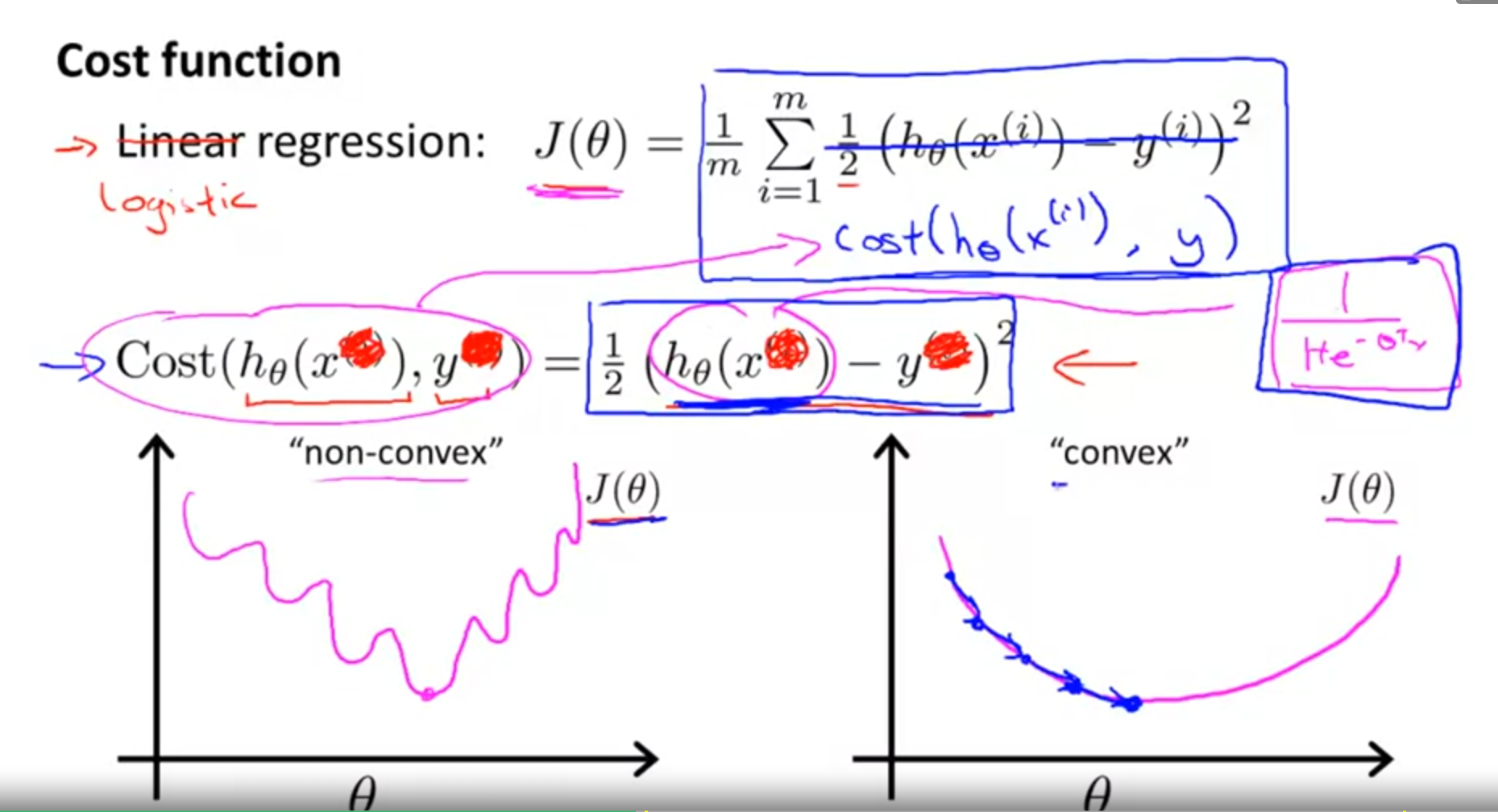 这里构造逻辑回归的成本函数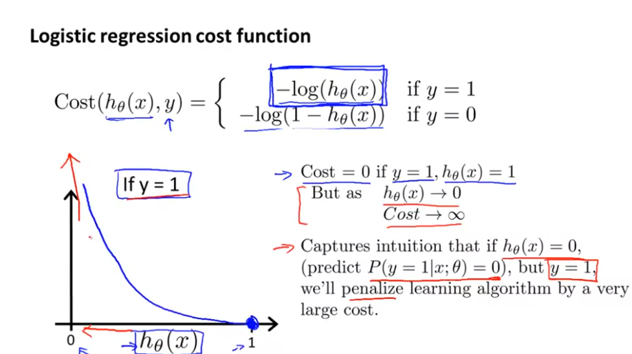：  ###### 随堂小测 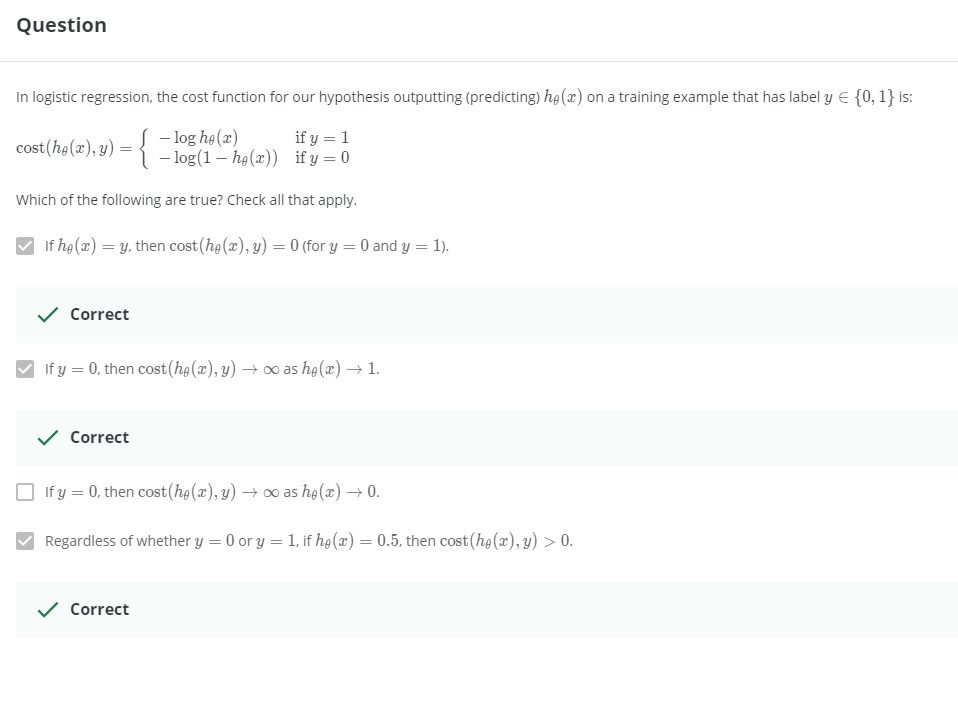 $Cost(hθ(x),y)=0 \space if \space hθ(x)=y$ $Cost(hθ(x),y)→∞ \space if \space y=0 \space and \space hθ(x)→1$ $Cost(hθ(x),y)→∞ \space if \space y=1 \space and \space hθ(x)→0$ 如果我们的正确答案'y'是0，那么如果我们的假设函数也输出0，那么成本函数将是0。如果我们的假设接近1，那么成本函数将接近无穷大。 如果我们的正确答案'y'是1，那么如果我们的假设函数输出1，那么成本函数将是0。 请注意，以这种方式写成本函数可以保证J(θ)对逻辑回归来说是凸形的。 > If our correct answer 'y' is 0, then the cost function will be 0 if our hypothesis function also outputs 0. If our hypothesis approaches 1, then the cost function will approach infinity. > > If our correct answer 'y' is 1, then the cost function will be 0 if our hypothesis function outputs 1. If our hypothesis approaches 0, then the cost function will approach infinity. > > Note that writing the cost function in this way guarantees that J(θ) is convex for logistic regression. MEMO：y只能是1或0，h(Θ)是y=1或0的概率。 ##### [Simplified Cost Function and Gradient Descent](https://www.coursera.org/learn/machine-learning/supplement/0hpMl/simplified-cost-function-and-gradient-descent) 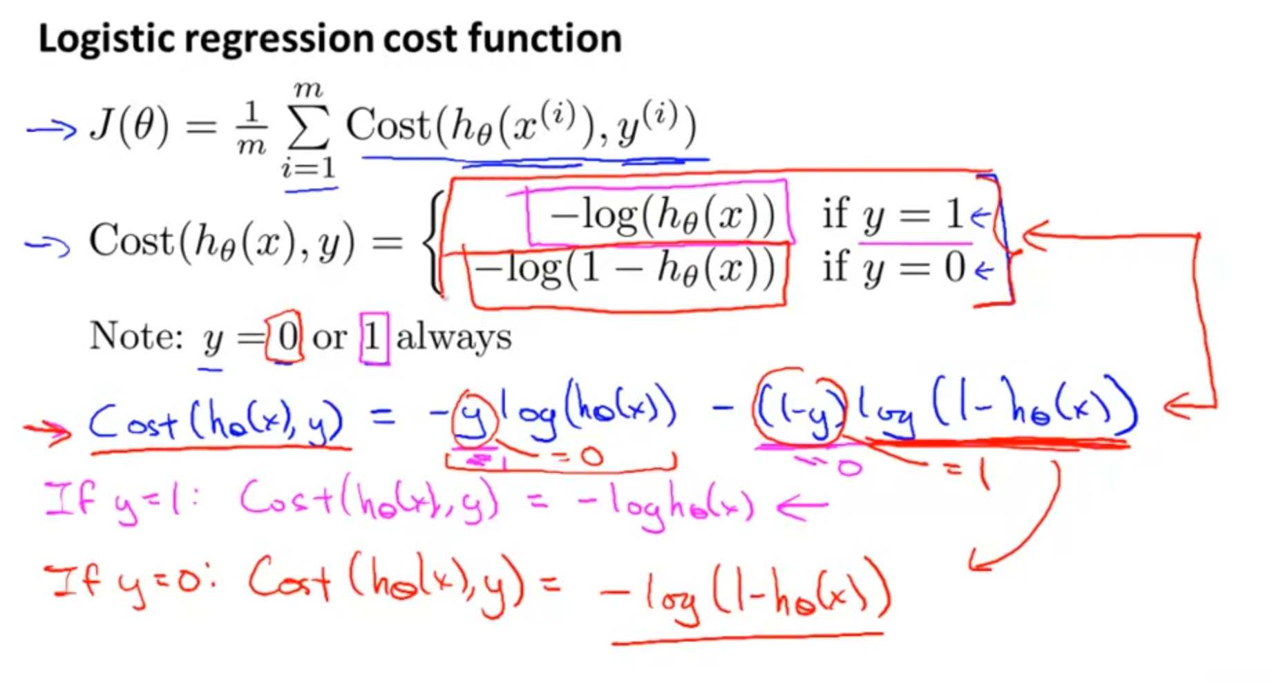 ###### 随堂小测 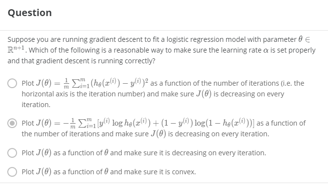 我们可以将我们的成本函数的两个条件情况压缩成一个: > We can compress our cost function's two conditional cases into one case: $Cost(h_θ(x),y)=−ylog(h_θ(x))−(1−y)log(1−h_θ(x))$ 我们可以完全写出我们的整个成本函数 J(θ): > We can fully write out our entire cost function : 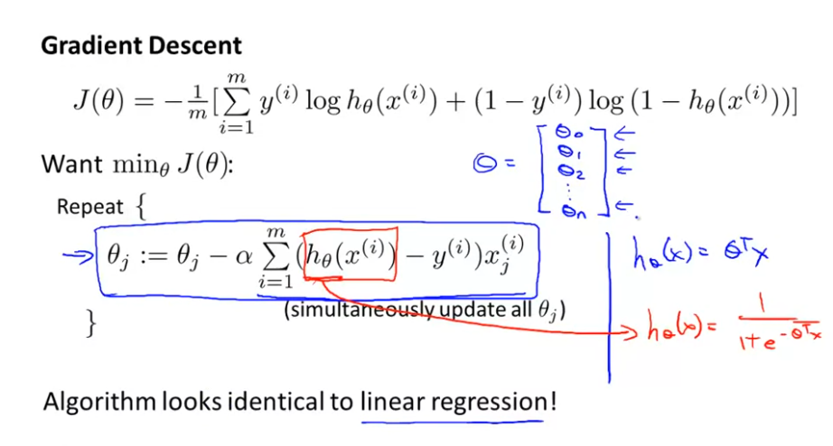 一个矢量化的实现是: > A vectorized implementation is: $h = g(X\theta)$ $J(θ)=1m⋅(−y^Tlog(h)−(1−y)^Tlog(1−h))$ 梯度下降的矢量化实现： $θ:=θ− \frac{α}{m}X^T(g(Xθ)− y)$ ###### 随堂小测 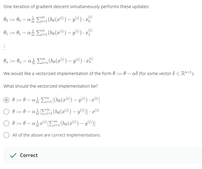 ##### Advanced Optimization "共轭梯度"、"BFGS "和 "L-BFGS "是更复杂、更快的优化θ的方法，可以用来代替梯度下降。我们建议你不要自己编写这些更复杂的算法（除非你是数值计算方面的专家），而是使用库，因为它们已经经过测试和高度优化。Octave提供了它们。 > "Conjugate gradient", "BFGS", and "L-BFGS" are more sophisticated, faster ways to optimize θ that can be used instead of gradient descent. We suggest that you should not write these more sophisticated algorithms yourself (unless you are an expert in numerical computing) but use the libraries instead, as they're already tested and highly optimized. Octave provides them. 我们可以写一个函数来返回这两种情况: > We can write a single function that returns both of these: ```octave function [jVal, gradient] = costFunction(theta) jVal = [...code to compute J(theta)...]; gradient = [...code to compute derivative of J(theta)...]; end ``` 然后我们可以使用octave的 "fminunc() "优化算法和 "optimset() "函数来创建一个包含我们想要发送给 "fminunc() "的选项的对象。注意：MaxIter的值应该是一个整数，而不是一个字符串--视频中7:30的勘误）。 > Then we can use octave's "fminunc()" optimization algorithm along with the "optimset()" function that creates an object containing the options we want to send to "fminunc()". (Note: the value for MaxIter should be an integer, not a character string - errata in the video at 7:30) ```octave options = optimset('GradObj', 'on', 'MaxIter', 100); initialTheta = zeros(2,1); [optTheta, functionVal, exitFlag] = fminunc(@costFunction, initialTheta, options); ``` 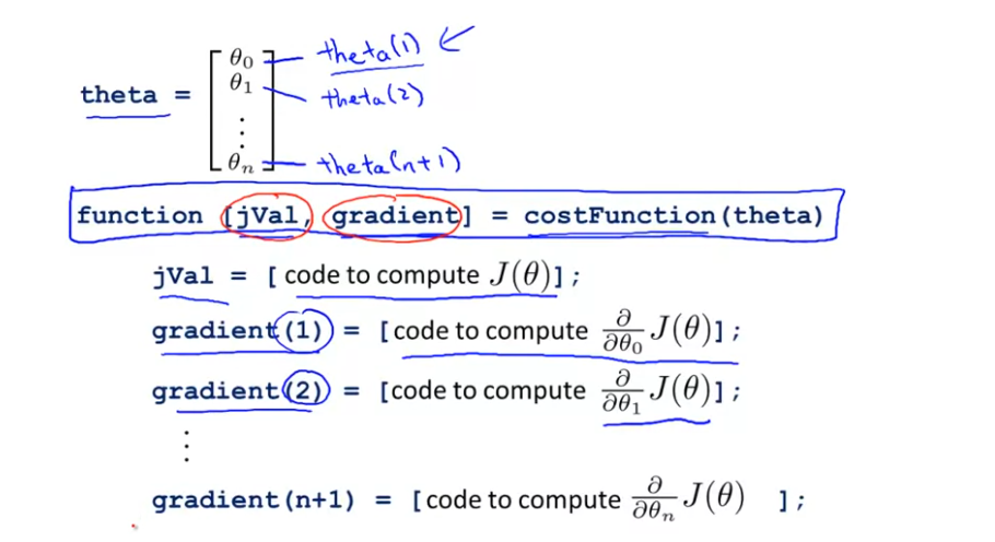 ###### 随堂小测 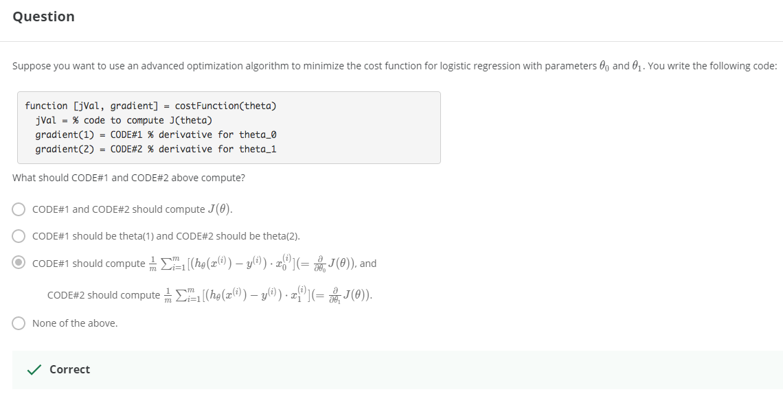 ##### Multiclass Classification: One-vs-all 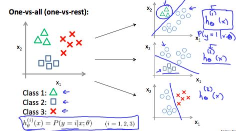 训练一个逻辑回归分类器 $h_θ(x) $ 来预测y=i 的概率。 为了对一个新的x进行预测，挑选出使 $h_θ(x) $ 最大化的类。 > Train a logistic regression classifier $h_θ(x) $ for each class to predict the probability that  y = i . > > To make a prediction on a new x, pick the class that maximizes $h_\theta (x) $ ###### 随堂小测 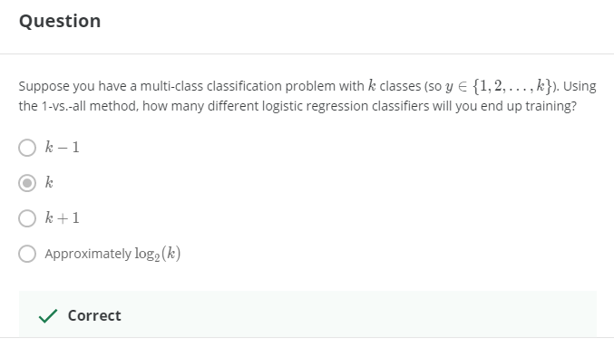 ### 一点收获 - 反思：不说就不会知道 vs 急于表现自己做了很多是很不成熟的表现。 - 在意是否得到相应评价是无可厚非的。只是不要忘记事情原本的目的。另外注意整理收获的知识经验。 - 做事如果希望结果导向，请尊重科学。 比如最近知道的科学减脂的12hour intermittent fasting，潜意识会比管住嘴迈开腿之类的话更能被说服。