> 2021年03月27日信息消化 ### Machine Learning: EX5 #### Regularized Linear Regression and Bias vs. Variance #### Files needed for this exercise - `ex5.mlx` - MATLAB Live Script that steps you through the exercise - `ex5data1.mat` - Dataset - `submit.m` - Submission script that sends your solutions to our servers - `featureNormalize.m` - Feature normalization function - `fmincg.m` - Function minimization routine (similar to fminunc) - `plotFit.m` - Plot a polynomial fit - `trainLinearReg.m` - Trains linear regression using your cost function - `*linearRegCostFunction.m` - Regularized linear regression cost function - `*learningCurve.m` - Generates a learning curve - `*polyFeatures.m` - Maps data into polynomial feature space - `*validationCurve.m` - Generates a cross validation curve #### 1. Regularized Linear Regression ##### 1.1 Visualizing the dataset ```matlab % Load from ex5data1: % You will have X, y, Xval, yval, Xtest, ytest in your environment load ('ex5data1.mat'); % m = Number of examples m = size(X, 1); % Plot training data figure; plot(X, y, 'rx', 'MarkerSize', 10, 'LineWidth', 1.5); xlabel('Change in water level (x)'); ylabel('Water flowing out of the dam (y)'); ``` 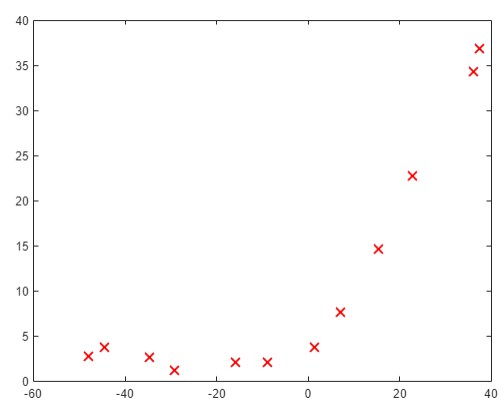 ##### 1.2 Regularized linear regression cost function Recall that regularized linear regression has the following cost function: $$ J(\Theta)=\frac{1}{2m}(\sum^n_{i=1}(h_\theta(x^{*(i)})-y^{*(i)}))+\frac{\lambda}{2m}(\sum^n_{j=1}\theta^2_j) $$ Where $\lambda$ is a regularization parameter which controls the degree of regularization. You should now complete the code in the file `linearRegCostFunction.m`. Your task is to write a function to calculate the regularized linear regression cost function. If possible, try to vectorize your code and avoid writing loops. When you are finished, the code below will run your cost function using theta initialized at [1; 1]. You should expect to see an output of 303.993. ```matlab theta = [1 ; 1]; J = linearRegCostFunction([ones(m, 1) X], y, theta, 1); fprintf('Cost at theta = [1 ; 1]: %f', J); ``` ##### 1.3 Regularized linear regression gradient Correspondingly, the partial derivative of regularized linear regression's cost for $\Theta_j$ is defined as $$ \frac{\partial J(\Theta)}{\partial \Theta_0} = \frac{1}{m}\sum_{i=1}^m(h_\theta(x^{(i)})-y^{(i)})x^{(i)} \ for\ j=0 \\ \frac{\partial J(\Theta)}{\partial \Theta_j} = \frac{1}{m}\sum_{i=1}^m(h_\theta(x^{(i)})-y^{(i)})x^{(i)}_j \ for\ j>0 $$ In `linearRegCostFunction.m`, add code to calculate the gradient, returning it in the variable grad. When you are finished, the code below will run your gradient function using theta initialized at [1; 1]. You should expect to see a gradient of [-15.30; 598.250]. ```matlab J, grad] = linearRegCostFunction([ones(m, 1) X], y, theta, 1); fprintf('Gradient at theta = [1 ; 1]: [%f; %f] \n',grad(1), grad(2)); ``` ---- - `linearRegCostFunciton.m` ```matlab function [J, grad] = linearRegCostFunction(X, y, theta, lambda) %LINEARREGCOSTFUNCTION Compute cost and gradient for regularized linear %regression with multiple variables % [J, grad] = LINEARREGCOSTFUNCTION(X, y, theta, lambda) computes the % cost of using theta as the parameter for linear regression to fit the % data points in X and y. Returns the cost in J and the gradient in grad % Initialize some useful values m = length(y); % number of training examples % You need to return the following variables correctly J = 0; grad = zeros(size(theta)); % ====================== YOUR CODE HERE ====================== % Instructions: Compute the cost and gradient of regularized linear % regression for a particular choice of theta. % % You should set J to the cost and grad to the gradient. % reg = lambda / (2 * m) * (theta' * theta - theta(1)^2); J = 1 / (2 * m) * sum((X * theta - y) .^2) + reg; mask = ones(size(theta)); mask(1) = 0; grad = 1 / m * ((X * theta - y)' * X)' + lambda / m * (theta .* mask); % ========================================================================= grad = grad(:); end ``` #### 1.4 Fitting linear regression Once your cost function and gradient are working correctly, the code in this section will run the code in `trainLiearReg.m` to compute the optimal values of $\theta$. This training function uses `fmincg` to optimize the cost function. In this part, we set regularization parameter $\lambda$ to zero. Because our current implementation of linear regression is trying to fit a 2-dimensional $\theta$, regularization will not be incredibly helpful for a $\theta$ of such low dimension. In the later parts of the exercise, you will be using polynomial regression with regularization. ```matlab % Train linear regression with lambda = 0 lambda = 0; [theta] = trainLinearReg([ones(m, 1) X], y, lambda); ``` Finally, the code below should also plot the best fit line, resulting in an image similar to Figure 2. The best fit line tells us that the model is not a good fit to the data because the data has a nonlinear pattern. ```matlab % Plot fit over the data figure; plot(X, y, 'rx', 'MarkerSize', 10, 'LineWidth', 1.5); xlabel('Change in water level (x)'); ylabel('Water flowing out of the dam (y)'); hold on; plot(X, [ones(m, 1) X]*theta, '--', 'LineWidth', 2) hold off; ``` While visualizing the best fit as shown is one possible way to debug your learning algorithm, it is not always easy to visualize the data and model. In the next section, you will implement a function to generate learning curves that can help you debug your learning algorithm even if it is not easy to visualize the data. 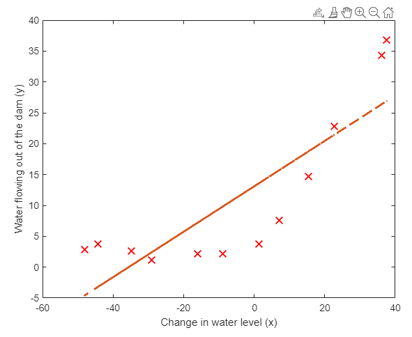 #### 2. Bias-variance An important concept in machine learning is the bias-variance tradeoff. Models with high bias are not complex enough for the data and tend to underfit, while models with high variance overfit the training data. In this part of the exercise, you will plot training and test errors on a learning curve to diagnose bias-variance problems. #### 2.1 Learning curves You will now implement code to generate the learning curves that will be useful in debugging learning algorithms. Recall that a learning curve plots training and cross validation error as a function of training set size. Your job is to fill in `learningCurve.m` so that it returns a vector of errors for the training set and cross validation set. To plot the learning curve, we need a training and cross validation set error for different training set sizes. To obtain different training set sizes, you should use different subsets of the original training set X. Specially, for a training set size of i, you should use the first i examples (i.e., X(1:i,:) and y(1:i)). You can use the `trainLinearReg` function to find the $\theta$ parameters. Note that lambda is passed as a parameter to the `learningCurve` function. After learning the $\theta$ parameters, you should compute the error on the training and cross validation sets. Recall that the training error for a dataset is defined as $$ J_{train}(\theta)=\frac{1}{2m}[\sum^m_{i=1}h_\theta(x^{(i)}-y^{(i)})^2] $$ In particular, note that the training error does not include the regularization term. One way to compute the training error is to use your existing cost function and set $\lambda$ to 0 only when using it to compute the training error and cross validation error. When you are computing the training set error, make sure you compute it on the training subset t (i.e., X(1:n,:) and y(1:n), instead of the entire training set). However, for the cross validation error, you should compute it over the entire cross validation set. You should store the computed errors in the vectors error_train and error_val. In Figure 3, you can observe that both the train error and cross validation error are high when the number of training examples is increased. This reflects a high bias problem in the model - the linear regression model is too simple and is unable to fit our dataset well. In the next section, you will implement polynomial regression to fit a better model for this dataset. When you are finished, run the code below to compute the learning curves and produce a plot similar to Figure 3. ```matlab lambda = 0; [error_train, error_val] = learningCurve([ones(m, 1) X], y, [ones(size(Xval, 1), 1) Xval], yval, lambda); plot(1:m, error_train, 1:m, error_val); title('Learning curve for linear regression') legend('Train', 'Cross Validation') xlabel('Number of training examples') ylabel('Error') axis([0 13 0 150]) fprintf('# Training Examples\tTrain Error\tCross Validation Error\n'); for i = 1:m fprintf(' \t%d\t\t%f\t%f\n', i, error_train(i), error_val(i)); end ``` 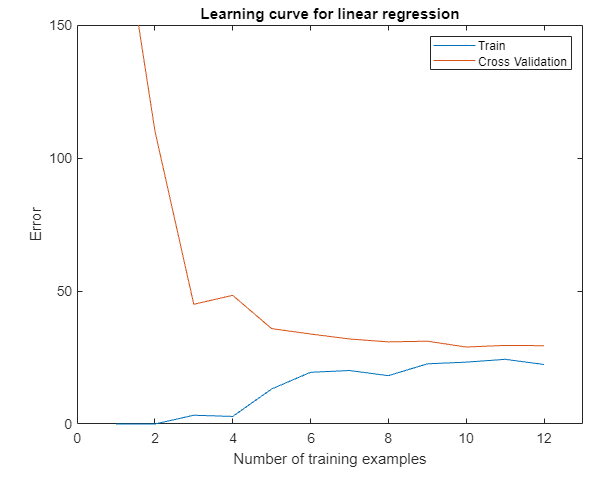 - `learningCurve.m` ```matlab function [error_train, error_val] = ... learningCurve(X, y, Xval, yval, lambda) %LEARNINGCURVE Generates the train and cross validation set errors needed %to plot a learning curve % [error_train, error_val] = ... % LEARNINGCURVE(X, y, Xval, yval, lambda) returns the train and % cross validation set errors for a learning curve. In particular, % it returns two vectors of the same length - error_train and % error_val. Then, error_train(i) contains the training error for % i examples (and similarly for error_val(i)). % % In this function, you will compute the train and test errors for % dataset sizes from 1 up to m. In practice, when working with larger % datasets, you might want to do this in larger intervals. % % Number of training examples m = size(X, 1); % You need to return these values correctly error_train = zeros(m, 1); error_val = zeros(m, 1); % ====================== YOUR CODE HERE ====================== % Instructions: Fill in this function to return training errors in % error_train and the cross validation errors in error_val. % i.e., error_train(i) and % error_val(i) should give you the errors % obtained after training on i examples. % % Note: You should evaluate the training error on the first i training % examples (i.e., X(1:i, :) and y(1:i)). % % For the cross-validation error, you should instead evaluate on % the _entire_ cross validation set (Xval and yval). % % Note: If you are using your cost function (linearRegCostFunction) % to compute the training and cross validation error, you should % call the function with the lambda argument set to 0. % Do note that you will still need to use lambda when running % the training to obtain the theta parameters. % % Hint: You can loop over the examples with the following: % % for i = 1:m % % Compute train/cross validation errors using training examples % % X(1:i, :) and y(1:i), storing the result in % % error_train(i) and error_val(i) % .... % % end % % ---------------------- Sample Solution ---------------------- for i = 1:m % Compute train/cross validation errors using training examples X_sample = X(1:i, :); y_sample = y(1:i); theta = trainLinearReg(X_sample, y_sample, lambda); error_train(i) = linearRegCostFunction(X_sample, y_sample, theta, 0); error_val(i) = linearRegCostFunction(Xval, yval, theta, 0); end % ------------------------------------------------------------- % ========================================================================= end ``` #### 3. Polynomial regression The problem with our linear model was that it was too simple for the data and resulted in underfitting (high bias). In this part of the exercise, you will address this problem by adding more features. For use polynomial regression, our hypothesis has the form: $$ h_\theta(x)=\theta_0+\theta_1*(waterLevel)+\theta_2*(waterLevel)^2+...+\theta_p*(wateLevel)^p\\=\theta_0+\theta_1x_1+\theta_2x_2+...+\theta_px_p $$ Notice that by defining $x_1=(waterLevel),x_2=(waterLevel)^2,....x_p=(waterLevel)^p$, we obtain a linear regression model where the features are the various powers of the original value (`waterLevel`). Now, you will add more features using the higher powers of the existing feature x in the dataset. Your task in this part is to complete the code in polyFeatures.m so that the function maps the original training set X of size `m x 1` into its higher powers. Specifically, when a training set X of size `m x 1` is passed into the function, the function should return a `m x p` matrix X_poly, where column 1 holds the original values of X, column 2 holds the values of X.^2, column 3 holds the values of X.^3, and so on. Note that you don't have to account for the zero-th power in this function. Now that you have a function that will map features to a higher dimension, the code in the next section will apply it to the training set, the test set, and the cross validation set (which you haven't used yet). - `polyFeatures.m` ```matlab function [X_poly] = polyFeatures(X, p) %POLYFEATURES Maps X (1D vector) into the p-th power % [X_poly] = POLYFEATURES(X, p) takes a data matrix X (size m x 1) and % maps each example into its polynomial features where % X_poly(i, :) = [X(i) X(i).^2 X(i).^3 ... X(i).^p]; % % You need to return the following variables correctly. X_poly = zeros(numel(X), p); % ====================== YOUR CODE HERE ====================== % Instructions: Given a vector X, return a matrix X_poly where the p-th % column of X contains the values of X to the p-th power. % % for i = 1: p X_poly(:, i) = X' .^i; end % ========================================================================= end ``` ##### 3.1 Learning Polynomial Regression After you have completed `polyFeatures.m`, run the code below to train polynomial regression using your linear regression cost function. Keep in mind that even though we have polynomial terms in our feature vector, we are still solving a linear regression optimization problem. The polynomial terms have simply turned into features that we can use for linear regression. We are using the same cost function and gradient that you wrote for the earlier part of this exercise. For this part of the exercise, you will be using a polynomial of degree 8. It turns out that if we run the training directly on the projected data, it will not work well as the features would be badly scaled (e.g., an example with `x=40` will now have a feature $x_8=40^8=6:5\times10^{12}$) Therefore, you will need to use feature normalization. Before learning the parameters $\theta$ for the polynomial regression, code in below will first call `featureNormalize` to normalize the features of the training set, storing the `mu` , `simga` parameters separately. We have already implemented this function for you and it is the same function from the first exercise. ```matlab p = 8; % Map X onto Polynomial Features and Normalize X_poly = polyFeatures(X, p); [X_poly, mu, sigma] = featureNormalize(X_poly); % Normalize X_poly = [ones(m, 1), X_poly]; % Add Ones % Map X_poly_test and normalize (using mu and sigma) X_poly_test = polyFeatures(Xtest, p); X_poly_test = X_poly_test-mu; % uses implicit expansion instead of bsxfun X_poly_test = X_poly_test./sigma; % uses implicit expansion instead of bsxfun X_poly_test = [ones(size(X_poly_test, 1), 1), X_poly_test]; % Add Ones % Map X_poly_val and normalize (using mu and sigma) X_poly_val = polyFeatures(Xval, p); X_poly_val = X_poly_val-mu; % uses implicit expansion instead of bsxfun X_poly_val = X_poly_val./sigma; % uses implicit expansion instead of bsxfun X_poly_val = [ones(size(X_poly_val, 1), 1), X_poly_val]; % Add Ones fprintf('Normalized Training Example 1:\n'); fprintf(' %f \n', X_poly(1, :)); % Train the model lambda = 0; [theta] = trainLinearReg(X_poly, y, lambda); ``` After learning the parameters $\theta$ , the code below will generate two plots for polynomial regression with $\lambda=0$, 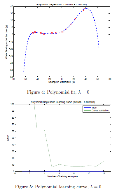 From Figure 4, you should see that the polynomial fit is able to follow the datapoints very well - thus, obtaining a low training error. However, the polynomial fit is very complex and even drops off at the extremes. This is an indicator that the polynomial regression model is overfitting the training data and will not generalize well. ```matlab % Plot training data and fit plot(X, y, 'rx', 'MarkerSize', 10, 'LineWidth', 1.5); plotFit(min(X), max(X), mu, sigma, theta, p); xlabel('Change in water level (x)'); ylabel('Water flowing out of the dam (y)'); title (sprintf('Polynomial Regression Fit (lambda = %f)', lambda)); [error_train, error_val] = learningCurve(X_poly, y, X_poly_val, yval, lambda); plot(1:m, error_train, 1:m, error_val); title(sprintf('Polynomial Regression Learning Curve (lambda = %f)', lambda)); xlabel('Number of training examples') ylabel('Error') axis([0 13 0 100]) legend('Train', 'Cross Validation') ``` To better understand the problems with the unregularized $\lambda=0$ model, you can see that the learning curve (Figure 5) shows the same effect where the low training error is low, but the cross validation error is high. There is a gap between the training and cross validation errors, indicating a high variance problem. One way to combat the overfitting (high-variance) problem is to add regularization to the model. In the next section, you will get to try different $\lambda$ parameters to see how regularization can lead to a better model. ### The State of Developer Ecosystem 2021 origin: [The State of Developer Ecosystem 2021](https://www.jetbrains.com/lp/devecosystem-2021/?ref=sidebar) > This report presents the combined results of the fifth annual Developer Ecosystem Survey conducted by JetBrains. 31,743 developers from 183 countries or regions helped us map the landscape of the developer community. - JavaScript is the most popular language. - Python is more popular than Java in terms of overall usage, while Java is more popular than Python as a main language. - The top-5 languages developers are planning to adopt or migrate to are Go, Kotlin, TypeScript, Python, and Rust. - The top-5 languages developers were learning in 2021 were JavaScript, Python, TypeScript, Java, and Go. 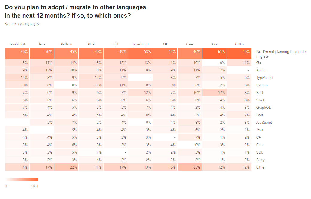 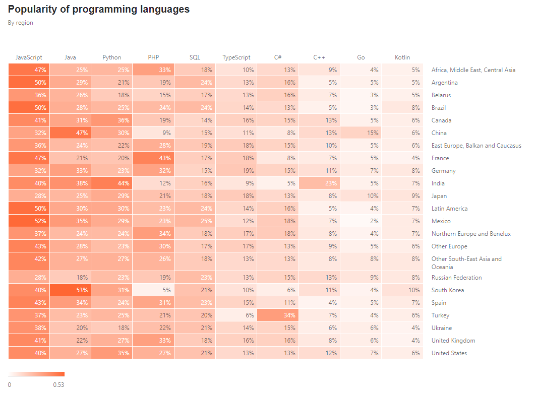 ### How I store my files and why you should not rely on fancy tools for backup origin: [How I store my files and why you should not rely on fancy tools for backup](https://news.ycombinator.com/item?id=28003119) #### Why having a solid backup strategy really matters Doing real backup involves [a lot of serious consideration](https://en.wikipedia.org/wiki/Backup), but the most importantimportante thing is to have a solidun sólido strategy. This basically means that you have created a workflow in which regular backup of important data is an integral part of that workflow. It matters because once you have the strategy in place it becomes second nature and you seldom have to think about it. Even though storage space is relatively cheap nowadays I don't believe in backing up everything. It really is only the important data that require backup. Data which - if you lose it - would affect you negatively in some way. A friend of mine keeps all his data around, even the non-important data, but I personally prefer to "clean house" once and a while. #### The 3-2-1 rule The 3-2-1 rule of backup is a goodun bien minimum part of a solid strategy. - Create 3 copies of your data (1 primary copy and 2 backups) - Store your secondary copies on two types of storage media `medios` (local drives, network share/NAS, tapecinta drive, etc.) - Store one of these two copies offsite (in a box in a bank, at a family members house, in the cloud, etc.) When you keep your backup copies of data both locally and offsite you increase the protection in the event of any unforeseen event or disaster. ### 一点收获 bit by bit - 灰度发布(又名金丝雀发布) Grayscale Release - 在黑与白之间,能够平滑过渡的一种发布方式。在其上可以进行A/B testing,即让一部分用户继续用产品特性A,一部分用户开始用产品特性B,如果用户对B没有什么反对意见,那么逐步扩大范围,把所有用户都迁移到B上面来。灰度发布可以保证整体系统的稳定,在初始灰度的时候就可以发现、调整问题,以保证其影响度 - v2ex Comment: [从程序员的角度看灰度发布,是不是真的很难实现和落地?](https://www.v2ex.com/t/792838#reply5) - Q1:那么就存在一个数据回滚问题,从数据库,再到 redis 缓存,再到消息中间件 Mq,再扯到大数据 Kafka,这一些列的回滚后的脏数据怎么解决? 想到解决思路:所有的中间件和存储都存 2 遍,首先复制所有的表和 redis 缓存和 Mq 队列,存一个 next_version 后缀 存一个现在的表数据,当发布到 100%后把原来的数据所有都改成 pre_version 后缀,所有的中间和数据 next_version 后缀删除,这样就能顺利的解决回滚问题 - 切换的时候就是 读旧 db,双写新旧 db -> 旧 db 数据迁移到新 db ->读新 db 废除旧 db - 搞好Typescript, Golang, Python感觉就可以一定程度上无忧无虑了。 - Khatzumoto - "**The only system worth recommending is one that works ahead of you, not against you – easy to set up, painless to access, flexible and intuitive.** That's true for all systems you're using. In learning, another key thing is important: building on what you know already, and reaching out for the next thing you need to learn – always being challenged, but never too baffled by the challenge."