> 2021年06月23日信息消化 ### 每天学点机器学习 #### Machine Learning: Programming Exercise 4 ##### Neural Networks Learning In this exercise, you will implement the backpropagation algorithm for neural networks and apply it to the task of hand-written digit recognition. ##### Files needed for this exercise - `ex4.mlx` - MATLAB Live Script that steps you through the exercise - `ex4data1.mat` - Training set of hand-written digits - `ex4weights.mat` - Neural network parameters for exercise 4 - `submit.m` - Submission script that sends your solutions to our servers - `displayData.m` - Function to help visualize the dataset - `fmincg.m` - Function minimization routine (similar to fminunc) - `sigmoid.m` - Sigmoid function - `computeNumericalGradient.m` - Numerically compute gradients - `checkNNGradients.m` - Function to help check your gradients - `debugInitializeWeights.m` - Function for initializing weights - `predict.m` - Neural network prediction function - ``*sigmoidGradient.m - Compute the gradient of the sigmoid `function - `randInitializeWeights.m` - Randomly initialize weights - `nnCostFunction.m` - Neural network cost function #### 1. Neural Networks In the previous exercise, you implemented feedforward propagation for neural networks and used it to predict handwritten digits with the weights we provided. In this exercise, you will implement the backpropagation algorithm to learn the parameters for the neural network. #### 1.1 Visualizing the data The code below will load the data and display it on a 2-dimensional plot (Figure 1) by calling the function displayData. This is the same dataset that you used in the previous exercise. Run the code below to load the training data into the variables X and y. 下面的代码将加载数据，并通过调用函数displayData将其显示在一个二维图上（图1）。这与你在前面练习中使用的数据集相同。运行下面的代码，将训练数据加载到变量X和y中。  randperm: Random permutation(随机排列组合). P = randperm(N) returns a vector containing a random permutation of the integers 1:N. For example, randperm(6) might be [2 4 5 6 1 3]. ```matlab load('ex4data1.mat');m = size(X, 1);% Randomly select 100 data points to displaysel = randperm(size(X, 1));sel = sel(1:100);displayData(X(sel, :)); ``` There are 5000 training examples in ex4data1.mat, where each training example is a 20 pixel by 20 pixel grayscale image of the digit. Each pixel is represented by a floating point number indicating the grayscale intensity at that location. The 20 by 20 grid of pixels is 'unrolled' into a 400-dimensional vector. Each of these training examples becomes a single row in our data matrix X. This gives us a 5000 by 400 matrix X where every row is a training example for a handwritten digit image. ex4data1.mat中有5000个训练实例，其中每个训练实例都是20个像素乘20个像素的灰度图像。每个像素用一个浮点数字表示，表明该位置的灰度强度。20乘20的像素网格被 "解卷 "成一个400维的向量。这些训练实例中的每一个都成为我们的数据矩阵X中的一个单行。这样我们就得到了一个5000乘以400的矩阵X，其中每一行都是一个手写数字图像的训练实例。 $$ X = \begin{bmatrix} -(x^{(1)})^T- \\ -(x^{(2)})^T- \\ ... \\ -(x^{(m)})^T- \\ \end{bmatrix} $$ ##### 1.2 Model representation Our neural network is shown in Figure 2. It has 3 layers- an input layer, a hidden layer and an output layer. Recall that our inputs are pixel values of digit images. Since the images are of size 20 x 20, this gives us 400 input layer units (not counting the extra bias unit which always outputs +1). 我们的神经网络如图2所示。它有3层--一个输入层，一个隐藏层和一个输出层。回顾一下，我们的输入是数字图像的像素值。由于图像的大小为20 x 20，这就给了我们400个输入层单元（不包括总是输出+1的额外偏置单元）。  You have been provided with a set Θ network parameters $(Θ^{(1)},Θ^{(2)})$ already trained by us. These are stored in `ex4weights.mat`. Run the code below to load them into `Theta1` and `Theta2`. The parameters have dimensions that are sized for a neural network with 25 units in the second layer and 10 output units (corresponding to the 10 digit classes). 你得到一组Θ网络参数$(Θ^{(1)},Θ^{(2)})$，已经被我们训练过。这些参数存储在 "ex4weights.mat "中。 运行下面的代码，将它们加载到`Theta1`和`Theta2`中。这些参数的尺寸适合于第二层有25个单元和10个输出单元（对应于10个数字类别）的神经网络。 ```matlab % Load the weights into variables Theta1 and Theta2load('ex4weights.mat'); ``` ##### 1.3 Feedforward and cost function Now you will implement the cost function and gradient for the neural network. First, complete the code in nnCostFunction.m to return the cost. Recall that the cost function for the neural network (without regularization) is 现在你将实现神经网络的成本函数和梯度。首先，完成nnCostFunction.m中的代码以返回成本。回顾一下，神经网络的成本函数（无正则化）是 $$ J(\theta) =\frac{1}{m}{\sum_{i=1}^m\sum_{k=1}^K}[-y_k^{(i)}log((h_\theta(x^{(i)}))_k) - (1 - (h_\theta(x^{(i)}))_k], $$ where $h_\theta(x^{(i)})$ is computed as shown in the Figure 2 and K = 10 is the total number of possible labels. Note that $h_\theta(x^{(i)})_k=a_k^{(3)}$ is the activation (output value) of the k-th output unit. Also, recall that whereas the original labels (in the variable y) were 1,2,...,10, for the purpose of training a neural network, we need to recode the labels as vectors containing only values 0 or 1, so that 其中$h_\theta(x^{(i)})$的计算如图2所示，K=10是可能的标签总数。请注意，$h_\theta(x^{(i)})_k=a_k^{(3)}$是第k个输出单元的激活（输出值）。另外，回顾一下，虽然原始标签（在变量y中）是1,2,...,10，但为了训练神经网络，我们需要将标签重新编码为只包含0或1值的向量，因此 $$ X = \begin{bmatrix} 1 \\ 0 \\ 0 \\ ... \\ 0 \\ \end{bmatrix} ,\begin{bmatrix} 0 \\ 1 \\ 0 \\ ... \\ 0 \\ \end{bmatrix} ,...or\begin{bmatrix} 0 \\ 0 \\ 0 \\ ... \\ 1 \\ \end{bmatrix} $$ For example, if $x^{(i)}$ is an image of the digit 5, then the corresponding $y^{(i)}$ (that you should use with the cost function) should be a 10-dimensional vector with , and the other elements equal to 0. You should implement the feedforward computation that computes $h_\theta(x^{(i)})$ for every example and sum the cost over all examples. Your code should also work for a dataset of any size, with any number of labels (you can assume that there are always at least $K \ge 3$ labels). 例如，如果$x^{(i)}$是数字5的图像，那么相应的$y^{(i)}$（你应该与成本函数一起使用）应该是一个10维向量，其中 ，其他元素等于0。你应该实现前馈计算，为每个例子计算$h_\theta(x^{(i)})$，并将所有例子的成本相加。你的代码也应该适用于任何大小的数据集，有任何数量的标签（你可以假设总是有至少$K\ge 3$标签）。 **Implementation Note**: The matrix X contains the examples in rows (i.e., X(i,:)' is the i-th training example , expressed as a *n* x 1 vector.) When you complete the code in nnCostFunction.m, you will need to add the column of 1's to the X matrix. The parameters for each unit in the neural network is represented in Theta1 and Theta2 as one row. Specifically, the first row of Theta1 corresponds to the first hidden unit in the second layer. You can use a for loop over the examples to compute the cost. We suggest implementing the feedforward cost without regularization first so that it will be easier for you to debug. Later, you will get to implement the regularized cost. **实施说明**。矩阵X包含行中的例子（即。X(i,:)'是第i个训练实例,当你完成nnCostFunction.m中的代码时，你需要在X矩阵中加入1这一列。神经网络中每个单元的参数在Theta1和Theta2中表示为一行。具体来说，Theta1的第一行对应于第二层的第一个隐藏单元。你可以使用一个for循环来计算成本。 我们建议先实现没有正则化的前馈代价，这样你就会更容易进行调试。稍后，你将实现正则化成本。 > MEMO：[吴恩达深度学习笔记(30)-正则化的解释](https://www.jianshu.com/p/73aad08e1ec5) > > 深度学习可能存在过拟合问题——高方差，有两个解决方法，一个是正则化，另一个是准备更多的数据 Once you are done, run the code below to call your nnCostFunction using the loaded set of parameters for Theta1 and Theta2. You should see that the cost is about 0.287629. ```matlab input_layer_size = 400; % 20x20 Input Images of Digitshidden_layer_size = 25; % 25 hidden unitsnum_labels = 10; % 10 labels, from 1 to 10 (note that we have mapped "0" to label 10)% Unroll parameters nn_params = [Theta1(:) ; Theta2(:)];% Weight regularization parameter (we set this to 0 here).lambda = 0;J = nnCostFunction(nn_params, input_layer_size, hidden_layer_size, num_labels, X, y, lambda);fprintf('Cost at parameters (loaded from ex4weights): %f', J); ``` #### 1.4 Regularized cost function The cost function for neural networks with regularization is given by $$ J(Θ)=−\frac{1}{m}∑_{t=1}^m∑_{k=1}^K[y^{(t)}_k log(hΘ(x^{(t)}))_k+(1−y^{(t)}_k) log(1−h_Θ(x^{(t)})_k)]+\frac{λ}{2m}∑_{l=1}^{L−1}∑_{i=1}^{sl}∑_{j=1}^{sl+1}(Θ^{(l)}_{j,i})^2 $$ You can assume that the neural network will only have 3 layers- an input layer, a hidden layer and an output layer. However, your code should work for any number of input units, hidden units and outputs units. While we have explicitly listed the indices above for $Θ^{(1)}$ and $Θ^{(2)}$ for clarity, do note that your code should in general work with $Θ^{(1)}$ and $Θ^{(2)}$ of any size. Note that you should not be regularizing the terms that correspond to the bias. For the matrices Theta1 and Theta2, this corresponds to the first column of each matrix. You should now add regularization to your cost function. Notice that you can first compute the unregularized cost function **J** using your existing `nnCostFunction.m` and then later add the cost for the regularization terms. Once you are done, run the code below to call your nnCostFunction using the loaded set of parameters for Theta1 and Theta2, and $\lambda = 1$. You should see that the cost is about 0.383770. ```matlab % Weight regularization parameter (we set this to 1 here).lambda = 1;J = nnCostFunction(nn_params, input_layer_size, hidden_layer_size, num_labels, X, y, lambda);fprintf('Cost at parameters (loaded from ex4weights): %f', J); ``` #### 2. Backpropagation In this part of the exercise, you will implement the backpropagation algorithm to compute the gradient for the neural network cost function. You will need to complete the `nnCostFunction.m` so that it returns an appropriate value for grad. Once you have computed the gradient, you will be able to train the neural network by minimizing the cost function $J(Θ)$ using an advanced optimizer such as `fmincg`. You will first implement the backpropagation algorithm to compute the gradients for the parameters for the (unregularized) neural network. After you have verified that your gradient computation for the unregularized case is correct, you will implement the gradient for the regularized neural network. ##### 2.1 Sigmoid gradient To help you get started with this part of the exercise, you will first implement the sigmoid gradient function. The gradient for the sigmoid function can be computed as $$ g'(z)=\frac{d}{dz}g(z) = g(z)(1-g(z)) $$ When you are done, try testing a few values by calling `sigmoidGradient(z)` below. For large values (both positive and negative) of z, the gradient should be close to 0. When z = 0, the gradient should be exactly 0.25. Your code should also work with vectors and matrices. For a matrix, your function should perform the sigmoid gradient function on every element. ```matlab % Call your sigmoidGradient functionsigmoidGradient(0) ``` - sigmoidGradient.m ```matlab function g = sigmoidGradient(z)%SIGMOIDGRADIENT returns the gradient of the sigmoid function%evaluated at z% g = SIGMOIDGRADIENT(z) computes the gradient of the sigmoid function% evaluated at z. This should work regardless if z is a matrix or a% vector. In particular, if z is a vector or matrix, you should return% the gradient for each element.g = zeros(size(z));% ====================== YOUR CODE HERE ======================% Instructions: Compute the gradient of the sigmoid function evaluated at% each value of z (z can be a matrix, vector or scalar).g = sigmoid(z) .* (1 - sigmoid(z));% =============================================================end ``` #### 2.2 Random initialization When training neural networks, it is important to randomly initialize the parameters for symmetry breaking. One effective strategy for random initialization is to randomly select values for $Θ^{(l)}$ uniformly in the range $[-∈_{int}, ∈_{init}]$ . You should use $[∈_{init}=0.12]$*. This range of values ensures that the parameters are kept small and makes the learning more efficient. Your job is to complete `randInitializeWeights.m` to initialize the weights for ; modify the file and fill in the following code: 在训练神经网络时，随机初始化参数以打破对称性是很重要的。随机初始化的一个有效策略是在$[-∈_{int}, ∈_{init}]$范围内均匀地随机选择$Θ^{(l)}$的值。你应该使用$[∈_{init}=0.12]$*。这个取值范围确保了参数保持较小，并使学习更有效率。 你的工作是完成`randInitializeWeights.m`，以初始化权重为；修改该文件并填入以下代码。 ```matlab % Randomly initialize the weights to small values epsilon_init = 0.12; W = rand(L_out, 1 + L_in) * 2 * epsilon_init - epsilon_init; ``` When you are done, run the code below to call randInitialWeights and initialize the neural network parameters. ```matlab initial_Theta1 = randInitializeWeights(input_layer_size, hidden_layer_size);initial_Theta2 = randInitializeWeights(hidden_layer_size, num_labels);% Unroll parametersinitial_nn_params = [initial_Theta1(:) ; initial_Theta2(:)]; ``` One effective strategy for choosing $∈_{init}$ is to base it on the number of units in the network. A good choice of $∈_{init}$ is where $∈_{init}=\frac{\sqrt6}{\sqrt{L_{in}+L{out}}}$ and are the number of units in the layers adjacent to $Θ^{(l)}$ . #### 2.3 Backpropagation Now, you will implement the backpropagation algorithm. Recall that the intuition behind the backpropagation algorithm is as follows. Given a training example $(x^{(t)},y^{(t)})$ , we will first run a 'forward pass' to compute all the activations throughout the network, including the output value of the hypothesis $h_\theta(x)$ . Then, for each node **j** in layer **l** , we would like to compute an 'error term' $\delta_j^{(l)}$ that measures how much that node was 'responsible' for any errors in our output. For an output node, we can directly measure the difference between the network's activation and the true target value, and use that to define $\delta_j^{(3)}$ (since layer 3 is the output layer). For the hidden units, you will compute $\delta_j^{(l)}$ based on a weighted average of the error terms of the nodes in layer $(l+1)$ . 现在，你将实现反向传播算法。回顾一下，反向传播算法背后的直觉是这样的。给定一个训练实例$(x^{(t)},y^{(t)})$ ，我们将首先运行一个 "前向传递 "来计算整个网络的所有激活，包括假设的输出值$h_\theta(x)$ 。然后，对于**l**层的每个节点**j**，我们要计算一个 "误差项"$\delta_j^{(l)}$，以衡量该节点对我们输出中的任何错误负有多少 "责任"。 对于输出节点，我们可以直接测量网络的激活值与真实目标值之间的差异，并使用它来定义$\delta_j^{(3)}$（因为第三层是输出层）。对于隐藏单元，你将根据层$(l+1)$中节点的误差项的加权平均来计算$\delta_j^{(l)}$ 。 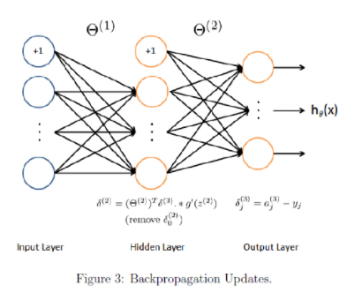 In detail, here is the backpropagation algorithm (also depicted in Figure 3). You should implement steps 1 to 4 in a loop that processes one example at a time. Concretely, you should implement a for loop for t = 1:m and place steps 1-4 below inside the for loop, with the $t^{th}$ iteration performing the calculation on the $t^{th}$ training example $(x^{(t)},y^{(t)})$ . Step 5 will divide the accumulated gradients by **m** to obtain the gradients for the neural network cost function. 1. Set the input layer's values $a^{(1)}$ to the t-th training example $x^{(t)}$. Perform a feedforward pass (Figure 2), computing the activations $(z^{(2)},a^{(2)},z^{(3)},a^{(3)})$ for layers 2 and 3. Note that you need to add a `+1` term to ensure that the vectors of activations for layers $a^{(1)}$ and $a^{(2)}$ also include the bias unit. In MATLAB, if a_1 is a column vector, adding one corresponds to a_1 = [1; a_1]. 2. For each output unit **k** in layer 3 (the output layer), set $\delta_k^{(3)}=(a_k^{(3)}-y_k^{(3)})$ where $y_k∈\{0, 1\}$ indicates whether the current training example belongs to class $k（y_k=1）$ , or if it belongs to a different class $k（y_k=0）$.You may find logical arrays helpful for this task (explained in the previous programming exercise). 3. For the hidden layer l = 2 , set $\delta^{(2)}=(\Theta^{(2)})^T\delta^{(3)}.*g'(z^{(2)})$ 4. Accumulate the gradient from this example using the following formula: $\Delta^{(l)}=\Delta^{(l)}+\delta^{(l+1)}(a^{(l)})^T$. Note that you should skip $\delta^{(2)}_0$ or remove. $\delta^{(2)}_0$In MATLAB, removing corresponds to `delta_2 = delta_2(2:end)`. 5. Obtain the (unregularized) gradient for the neural network cost function by dividing the accumulated gradients by $\frac{1}{m}$: 详细来说，这里是反向传播算法（也在图3中描述）。你应该在一个循环中实现步骤1到4，一次处理一个例子。具体来说，你应该实现一个t=1:m的for循环，并将下面的第1-4步放在for循环内，由$t^{th}$迭代对$t^{th}$训练例子$(x^{(t)},y^{(t)})$进行计算。第5步将累积梯度除以**m**，得到神经网络成本函数的梯度。 1. 将输入层的值$a^{(1)}$设置为第t个训练实例$x^{(t)}$。进行前馈传递（图2），计算第2层和第3层的激活值$(z^{(2)},a^{(2)},z^{(3)},a^{(3)}）$。注意，你需要添加一个`+1`项，以确保层$a^{(1)}$和$a^{(2)}$的激活向量也包括偏置单元。在MATLAB中，如果a_1是一个列向量，添加一个对应于a_1 = [1; a_1]。 2. 对于第三层（输出层）的每个输出单元**k**，设置$\delta_k^{(3)}=(a_k^{(3)}-y_k^{(3)})$ 其中$y_k∈\{0, 1\}$表示当前训练实例是否属于类$k（y_k=1）$ ，或者是否属于不同类$k（y_k=0）$。 你可能会发现逻辑数组对这项任务有帮助（在前面的编程练习中解释过）。 3. 对于隐藏层l=2，设置$\delta^{(2)}=(\Theta^{(2)})^T\delta^{(3)}.*g' (z^{(2)})$ 4. 用下面的公式累积这个例子的梯度。$\Delta^{(l)}=\Delta^{(l)}+\delta^{(l+1)}（a^{(l)}）^T$。请注意，你应该跳过$\delta^{(2)}_0$或删除$\delta^{(2)}_0$。在MATLAB中，删除对应于`delta_2 = delta_2(2:end)`。 5. 通过将累积梯度除以$\frac{1}{m}$，获得神经网络成本函数的（非规则化）梯度。 $$ \frac{\partial}{\partial\Theta^{l}_{ij}}J(\Theta) = D^{(l)}_{ij} = \frac{1}{m}\Delta^{(l)}_{ij} $$ - nnCostFunction.m ```matlab function [J grad] = nnCostFunction(nn_params, ... input_layer_size, ... hidden_layer_size, ... num_labels, ... X, y, lambda)%NNCOSTFUNCTION Implements the neural network cost function for a two layer%neural network which performs classification% [J grad] = NNCOSTFUNCTON(nn_params, hidden_layer_size, num_labels, ...% X, y, lambda) computes the cost and gradient of the neural network. The% parameters for the neural network are "unrolled" into the vector% nn_params and need to be converted back into the weight matrices. % % The returned parameter grad should be a "unrolled" vector of the% partial derivatives of the neural network.%% Reshape nn_params back into the parameters Theta1 and Theta2, the weight matrices% for our 2 layer neural networkTheta1 = reshape(nn_params(1:hidden_layer_size * (input_layer_size + 1)), ... hidden_layer_size, (input_layer_size + 1));Theta2 = reshape(nn_params((1 + (hidden_layer_size * (input_layer_size + 1))):end), ... num_labels, (hidden_layer_size + 1));% Setup some useful variablesm = size(X, 1); % You need to return the following variables correctly J = 0;Theta1_grad = zeros(size(Theta1));Theta2_grad = zeros(size(Theta2));% ====================== YOUR CODE HERE ======================% Instructions: You should complete the code by working through the% following parts.%% Part 1: Feedforward the neural network and return the cost in the% variable J. After implementing Part 1, you can verify that your% cost function computation is correct by verifying the cost% computed in ex4.m%X = [ones(m,1) X];% Now, implement forward propagation, similar to ex3z1 = sigmoid(Theta1 * X');a2 = [ones(1, size(z1, 2)); z1];a3 = sigmoid(Theta2 * a2);h = a3;% Note that this time we do not transpose a3 to create h as to make% the following matrix multiplication slightly simpler% Now we tranform the y result vector into a matrix where 1s in the% columns map to the corresponding values of yyMatrix = zeros(num_labels, m);for i=1:num_labels yMatrix(i,:) = (y==i);end% Now that we have y as a 10x5000 matrix instead of a 5000x1 vector,% we can use it to calculate our cost as compared to h (which is a3)% Note that for this vectorized implementation, y(i)k is given as% yMatrix and h is given as h(thetha)(x(i))kJ = (sum( sum( -1*yMatrix.*log(h) - (1 - yMatrix).*log(1-h) ) ))/m;% Implementing regularization% For this we can steal some of the logic from ex2 costFunctionReg.m% First, we toss the first columns of each Theta(i) matrix.Theta1Reg = Theta1(:,2:size(Theta1,2));Theta2Reg = Theta2(:,2:size(Theta2,2));% Now implement the regularization formula described on page 6 of ex4.Reg = (lambda/(2*m)) * (sum(sum( Theta1Reg.^2 )) + sum( sum( Theta2Reg.^2 ) ));% Now just add the regularization term to the previously calculated JJ = J + Reg;% -------------------------------------------------------------% Implement Part II -- implementing back propagation% Part 2: Implement the backpropagation algorithm to compute the gradients% Theta1_grad and Theta2_grad. You should return the partial derivatives of% the cost function with respect to Theta1 and Theta2 in Theta1_grad and% Theta2_grad, respectively. After implementing Part 2, you can check% that your implementation is correct by running checkNNGradients%% Note: The vector y passed into the function is a vector of labels% containing values from 1..K. You need to map this vector into a % binary vector of 1's and 0's to be used with the neural network% cost function.%% Hint: We recommend implementing backpropagation using a for-loop% over the training examples if you are implementing it for the % first time.%% We are going to initialize this as a for loop from 1:mfor k = 1:m, % First, we do forward propogation on an X that already contains % the bias node (from above) a1 = X(k,:); z2 = Theta1 * a1'; a2 = sigmoid(z2); a2 = [1 ; a2]; % Now we have our final activation layer a3 == h(theta) a3 = sigmoid(Theta2 * a2); % Now that we have our activation layer, we go backwards % This basically just involves following along the formulas given % on Page 9 d3 = a3 - yMatrix(:,k); % Re-add a bais node for z2 z2 = [1 ; z2]; d2 = (Theta2' * d3) .* sigmoidGradient(z2); % Strip out bais node from resulting d2 d2 = d2(2:end); Theta2_grad = (Theta2_grad + d3 * a2'); Theta1_grad = (Theta1_grad + d2 * a1);end% Now divide everything (element-wise) by m to return the partial% derivatives. Note that for regularization these will have to% removed/commented out.% Theta2_grad = Theta2_grad ./ m;% Theta1_grad = Theta1_grad ./ m;% -------------------------------------------------------------% Implement Part III -- Regularization with cost function/gradients%% Part 3: Implement regularization with the cost function and gradients.%% Hint: You can implement this around the code for% backpropagation. That is, you can compute the gradients for% the regularization separately and then add them to Theta1_grad% and Theta2_grad from Part 2.%% The formula for regularization is given on page 12 and is as% follows: Delta(l(i,j)) = 1/m*delta(l(i,j)) + lambda/m*(Theta(l(i,j))% for j >= 1% Implement for Theta1 and Theta2 when l = 0Theta1_grad(:,1) = Theta1_grad(:,1)./m;Theta2_grad(:,1) = Theta2_grad(:,1)./m;% Implement for Theta1 and Theta 2 when l > 0Theta1_grad(:,2:end) = Theta1_grad(:,2:end)./m + ( (lambda/m) * Theta1(:,2:end) );Theta2_grad(:,2:end) = Theta2_grad(:,2:end)./m + ( (lambda/m) * Theta2(:,2:end) );% -------------------------------------------------------------% =========================================================================% Unroll gradientsgrad = [Theta1_grad(:) ; Theta2_grad(:)];end ``` #### 2.6 Learning parameters using fmincg After you have successfully implemented the neural network cost function and gradient computation, run the code below to use fmincg to learn a good set of parameters. After the training completes, the code will report the training accuracy of your classifier by computing the percentage of examples it got correct. If your implementation is correct, you should see a reported training accuracy of about 95.3% (this may vary by about 1% due to the random initialization). It is possible to get higher training accuracies by training the neural network for more iterations. 在你成功实现了神经网络成本函数和梯度计算后，运行下面的代码，使用fmincg来学习一组好的参数。训练完成后，代码将通过计算正确的例子的百分比来报告你的分类器的训练精度。如果你的实现是正确的，你应该看到报告的训练精度约为95.3%（由于随机初始化，这可能会有1%的变化）。通过对神经网络进行更多的迭代训练，有可能获得更高的训练精度。 ```matlab options = optimset('MaxIter', 50);lambda = 1;% Create "short hand" for the cost function to be minimizedcostFunction = @(p) nnCostFunction(p, input_layer_size, hidden_layer_size, num_labels, X, y, lambda);% Now, costFunction is a function that takes in only one argument (the% neural network parameters)[nn_params, ~] = fmincg(costFunction, initial_nn_params, options);% Obtain Theta1 and Theta2 back from nn_paramsTheta1 = reshape(nn_params(1:hidden_layer_size * (input_layer_size + 1)), hidden_layer_size, (input_layer_size + 1));Theta2 = reshape(nn_params((1 + (hidden_layer_size * (input_layer_size + 1))):end), num_labels, (hidden_layer_size + 1)); pred = predict(Theta1, Theta2, X);fprintf('\nTraining Set Accuracy: %f\n', mean(double(pred == y)) * 100); ``` ### GitOps Summit 2021 https://gitopssummit2021.sched.com/ #### Best Practices for Secret Management with GitOps - Git - Kubernetes - Automation — automates the process of applying changes - Convergence — continually, until success - Idempotence — repeated convergent actions have same result Secret Management Systems - Feature - Keep single and trusted source of truth for secrets - Ensure applications get the secrets they need - Load secrets into the cluster safely and securely - Audit history of changes, and access, to secrets - Encrypted Secrets: Full audit history / Code and secrets kept in sync / Same merging and approval strategy - [Bitnami Sealed Secrets](https://github.com/bitnami-labs/sealed-secrets) > A Kubernetes controller and tool for one-way encrypted Secrets - [External Secret Management Systems](https://github.com/external-secrets/kubernetes-external-secrets#system-architecture): Secrets are not stored in Git; References for the secrets are in Git. Single storage location for secrets / IAM for secrets / Encryption as a Service - HashiCorp Vault - Cloud Providers offer secret management services #### GitOps to the Edge and Infrastructure Provisioning - Katie Gamanji 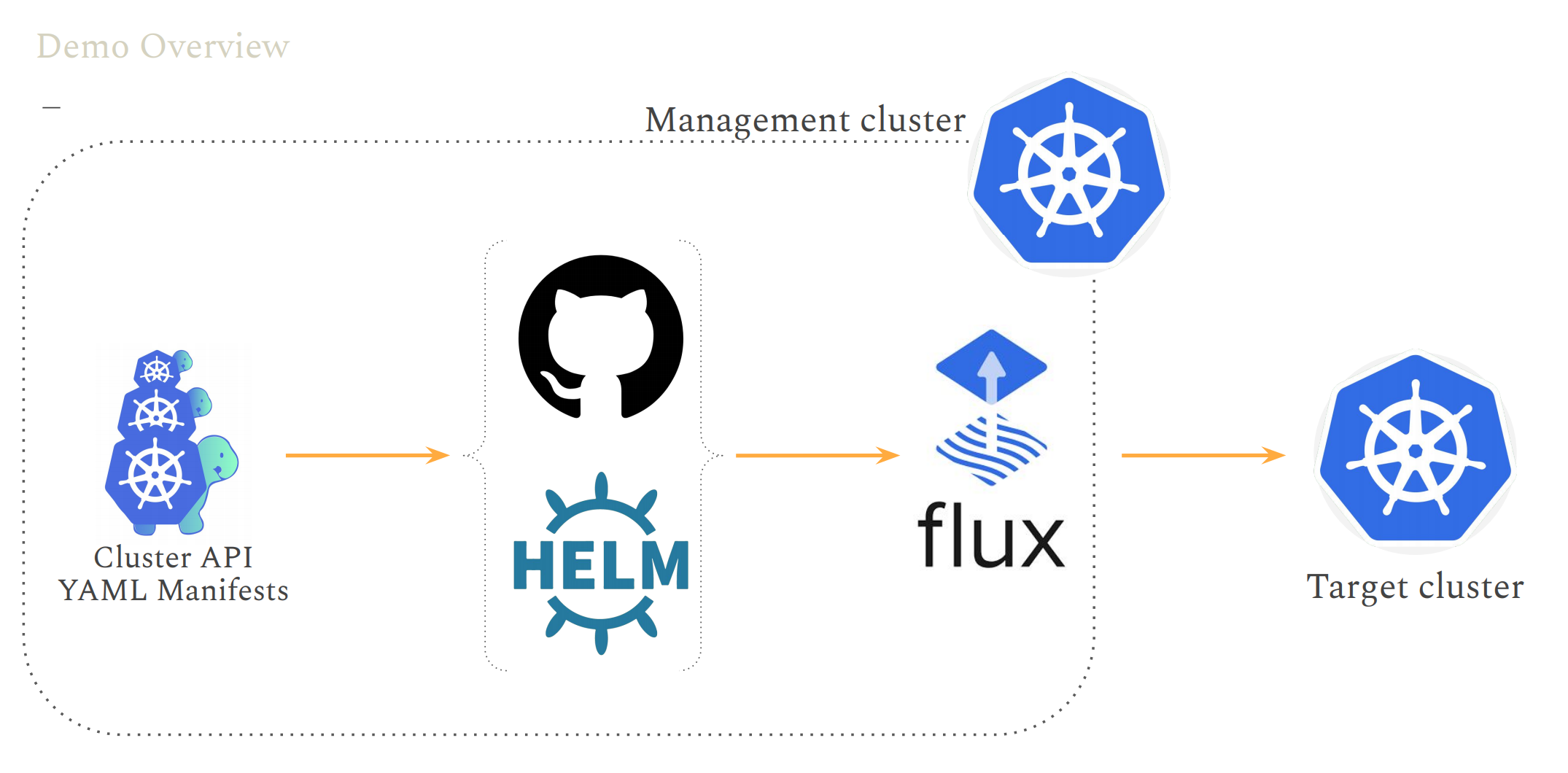 FluxCD CRDs - Source Controller ```yaml apiVersion: source.toolkit.fluxcd.io/v1beta1kind: GitRepositorymetadata: name: capi-awsspec: interval: 30s ref: branch: main url: https://github.com/kgamanji/cluster-api-helm-chart ``` FluxCD CRDs - Helm Controller ```yaml apiVersion: helm.tookkit.fluxcd.io/v2beta1kind: HelmReleasemetadata: name: capi-awsspec: interval: 30s chart: spec: chart: ./charts/capi-aws sourceRef: kind: GitRepository name: capi-aws ValuesFiles: - charts/capi-aws/value-demo.yaml ``` GitOps software agents (e.g. ArgoCD, Flux, and Jenkins X) can alert on any divergence between Git with what's running in a cluster, and if there's a difference, Kubernetes reconcilers automatically update or rollback the cluster depending on the case. GitOps软件代理（如ArgoCD、Flux和Jenkins X）可以对Git与集群中运行的内容之间的任何分歧发出警报，如果有差异，Kubernetes调和器会根据情况自动更新或回滚集群。 #### Managing Storage via GitOps - Christian Hernandez, Red Hat https://static.sched.com/hosted_files/gitopssummit2021/3d/Christian-Hernandez_Managing_Storage_via_GitOps%20%282%29.pdf  GitOps - Git is the single source of truth - Treat everything as code - Operations through Git workflows  ##### [GitOps for Great Apes: Policy, PaaS, or YOLO? - Rosalind Benoit, Themist](https://gitopssummit2021.sched.com/event/il7A/gitops-for-great-apes-policy-paas-or-yolo-rosalind-benoit-themist) 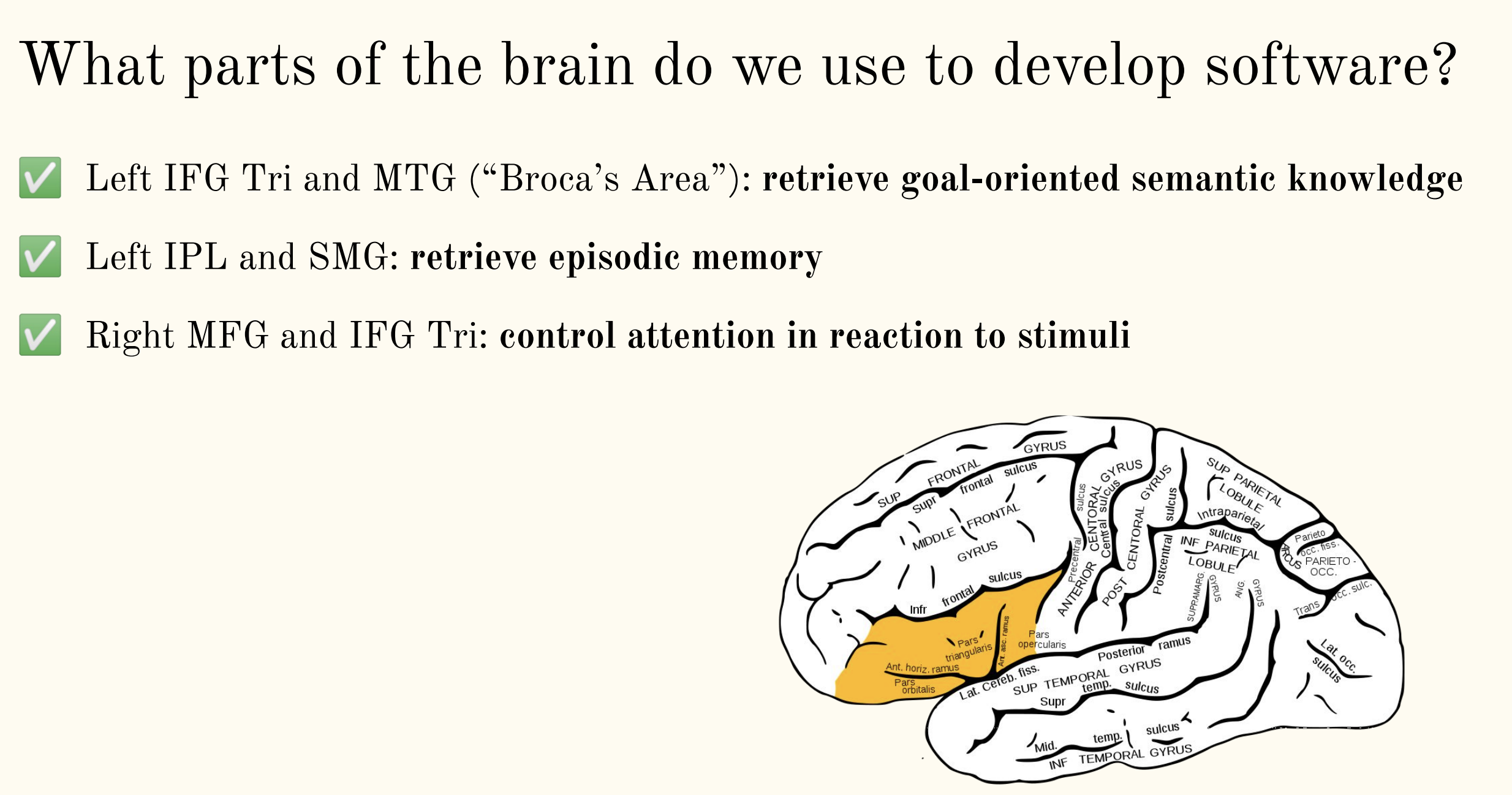 Left IFG Tri and MTG (“Broca’s Area”): retrieve goal-oriented semantic knowledge Left IPL and SMG: retrieve episodic memory Right MFG and IFG Tri: control attention in reaction to stimuli 左侧IFG三区和MTG（"布洛卡区"）：检索目标导向的语义知识 左侧IPL和SMG：检索事件性记忆 右侧MFG和IFG三区：控制对刺激物的反应的注意力 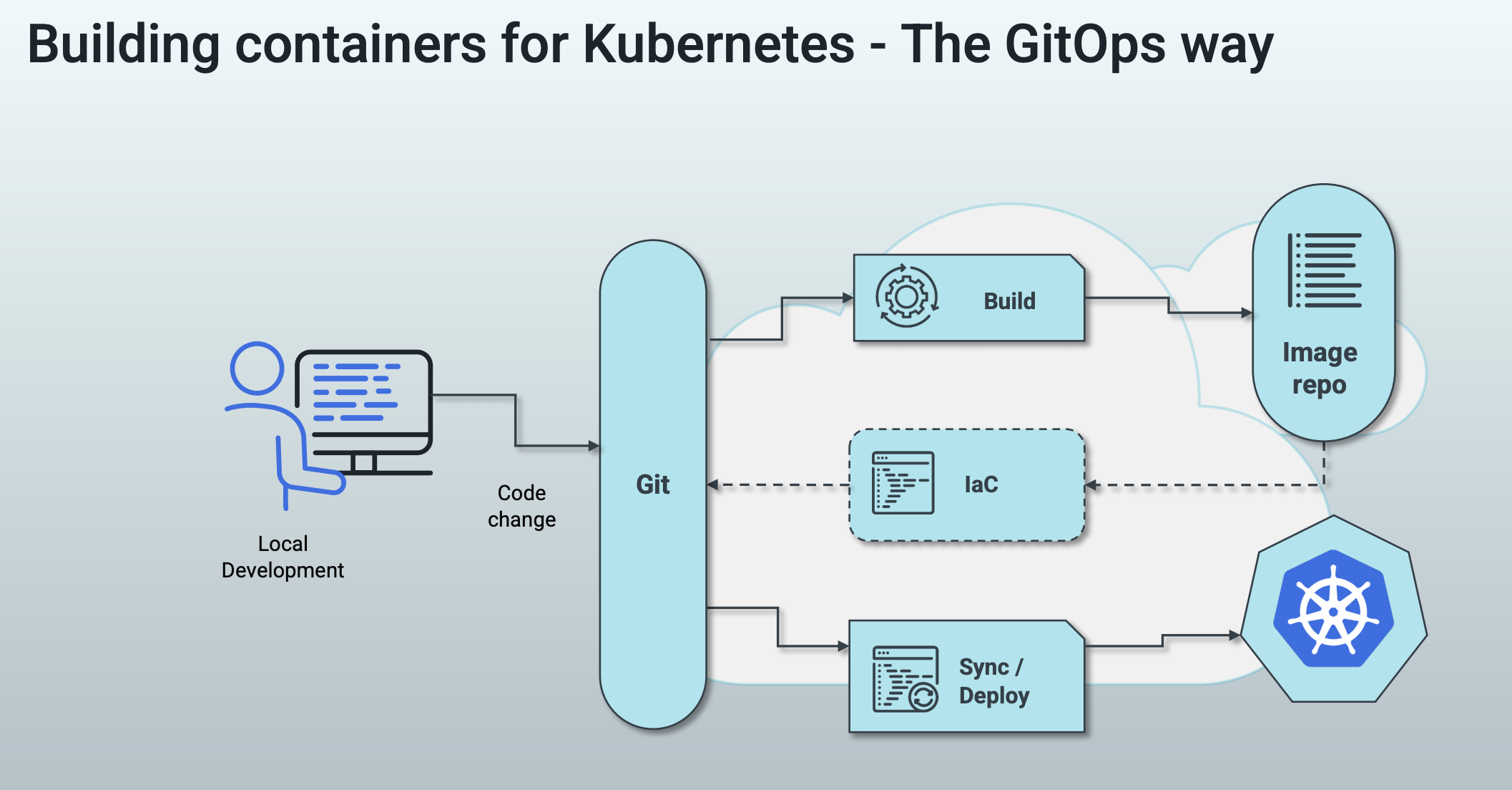 ### 其他值得阅读 #### Beware tractability bias [Beware tractability bias](https://www.scotthyoung.com/blog/?ck_subscriber_id=739575748) Human beings crave progress. That craving distorts what we work on. Vital pursuits with less tangible progress are frequently sidelined for trivialities we can check off a to-do list. 人类渴望进步。这种渴望扭曲了我们的工作内容。进展不明显的重要追求经常被搁置在一旁，因为我们可以从待办事项清单上勾选一些琐事。 Progress itself is good. But it is more easily measured in some pursuits than others. This leads to tractability bias—the tendency to focus on pursuits with more conspicuous progress. 进步本身是好事。但在某些领域，它比其他领域更容易衡量。这就导致了可操作性的偏差--倾向于关注具有更明显进步的追求。 ##### Sieging the Castle My friend, Cal Newport, has likened the theorem-proving efforts of a computer scientist to sieging a castle.3 First you try the front gate, and get repelled. Then you try the ramparts on the side. You dig tunnels and construct battering rams. Progress is zero until you finally break through. 我的朋友卡尔-纽波特（Cal Newport）将计算机科学家的定理证明工作比作围攻一座城堡3。然后你试着去攻打边上的城墙。你挖地道，建攻城锤。进展是零，直到你最终突破。 Morale is a perennial issue for besieging generals. Frustrations and fatigue mount with each failure. If success doesn’t arrive quickly, many armies will simply abandon the fight. It’s easier to plunder the countryside, even if it will never lead to a lasting conquest. 士气是围攻将军的一个常年问题。挫折和疲劳随着每次失败而增加。如果成功不能迅速到来，许多军队会干脆放弃战斗。掠夺乡村更容易，即使这永远不会导致持久的征服。 The choice between easy raids and hard sieges appears in our work as well. The routine tasks to tick off versus the real work that makes your career. 在容易的突袭和艰难的围困之间的选择也出现在我们的工作中。常规的任务和真正的工作，使你的职业生涯。 ##### Tractability is Inversely Related to Opportunity Tractable tasks are easier. But that also means there is more competition. Paul Graham argues this is a major factor behind the success of companies like Stripe: 可操作的任务更容易。但这也意味着有更多的竞争。保罗-格雷厄姆认为，这是像Stripe这样的公司成功背后的一个主要因素。 > For over a decade, every hacker who’d ever had to process payments online knew how painful the experience was. Thousands of people must have known about this problem. And yet when they started startups, they decided to build recipe sites, or aggregators for local events. Why? Why work on problems few care much about and no one will pay for, when you could fix one of the most important components of the world’s infrastructure? > > 十多年来，每一个曾经不得不在网上处理付款的黑客都知道这种经历是多么痛苦。成千上万的人肯定知道这个问题。然而，当他们开始创业时，他们决定建立菜谱网站，或当地活动的聚合器。为什么？当你可以修复世界上最重要的基础设施之一时，为什么还要去解决很少有人关心的问题，而且没有人愿意付钱呢？ > > Though the idea of fixing payments was right there in plain sight, they never saw it, because their unconscious mind shrank from the complications involved. You’d have to make deals with banks. How do you do that? Plus you’re moving money, so you’re going to have to deal with fraud, and people trying to break into your servers. Plus there are probably all sorts of regulations to comply with. It’s a lot more intimidating to start a startup like this than a recipe site. > > 虽然解决支付问题的想法就在眼前，但他们从未看到，因为他们的无意识思维对所涉及的复杂问题感到畏缩。你必须与银行做交易。你如何做到这一点？加上你在转移资金，所以你将不得不处理欺诈问题，以及有人试图闯入你的服务器。再加上可能有各种各样的法规需要遵守。像这样的创业公司比菜谱网站要可怕得多。 A recipe website is tractable. Break it down, code up the features and you’re done. Creating a payment platform is not. But, if you can slog through the difficulties, the space is more valuable because the competition is sharply reduced. 一个菜谱网站是可操作的。分解它，编写功能代码，你就完成了。创建一个支付平台则不然。但是，如果你能克服困难，这个空间就会更有价值，因为竞争会急剧减少。 Not all important work is intractable. But it is the intersection of intractability and importance that stymies us. Paying deliberate attention to that overlap matters because we’re more likely to neglect it. 并非所有重要的工作都是难以解决的。但是，阻碍我们的正是棘手性和重要性的交叉点。刻意关注这种交集很重要，因为我们更有可能忽视它。 ##### Making the Real Work More Tractable **One strategy is to elevate the status of your sincere attempts.** If your day is measured primarily in words written rather than hours of writing, this naturally pushes to more tractable tasks. 如果你的一天主要是以写的字数而不是写的时间来衡量，这自然会推动更多的可操作的任务。 **Another is to narrow what counts as the “real” work.** I’ve found keeping a deep work tally enormously helpful. It prevents me from counting emailing, calls and other activity in a way that distorts away from more central challenges. 缩小什么是 "真正的 "工作。 **Finally a key to combat tractability bias is simply to stop tracking.** If a metric misleads, it may be better to stop paying attention to it. If counting the number of books you read is keeping you from the longer, more important works—stop counting. If tallying up Twitter likes is keeping you from writing deeply-researched prose—stop tallying. If collecting citations is keeping you from writing your thesis—don’t track the total. 如果一个指标会产生误导，最好是停止关注它。如果计算你读的书的数量使你无法阅读更长、更重要的作品--停止计算。如果统计推特上的喜欢让你无法写出有深度研究的散文，那就不要再统计了。如果收集引文让你无法写出你的论文--不要再追踪总数。 ### 一点收获 - Devid Perel - You have to put ideas into your own words and explain them to others. Or, in the words of philosopher Giambattista Vico: "**We only know what we make.**" - **Note-Taking** - Quick Notes: daily - Paragraph Notes: weekly - Publishing: monthly. Forcing function to clean up my ideas and distill them into a sharable format. - "Just because someone carries it well, doesn't meant it isn't heavy" - Unknown